Introduction to FASSTER • fasster

library(fasster)
#> Loading required package: fabletools
#> Registered S3 method overwritten by 'tsibble':
#>   method               from 
#>   as_tibble.grouped_df dplyr

Overview

FASSTER (Forecasting with Additive Switching of Seasonality, Trend and Exogenous Regressors) is a state space model designed for forecasting time series with complex multiple seasonality patterns. The model addresses common limitations in existing approaches by providing:

Flexibility: Modular specification of trend, seasonality, and ARMA components
State switching: Different seasonal patterns for different categories (e.g., weekdays vs. weekends)
Exogenous regressors: Natural support for external variables
Speed: Efficient estimation using the Kalman filter
Decomposition: Model-based decomposition reveals underlying patterns

When to use FASSTER

FASSTER is particularly useful for time series with:

Multiple seasonal patterns that change based on categories or conditions
Irregular switching between patterns (e.g., working days vs. holidays)
High-frequency data where traditional methods are too slow
Missing values that need to be handled gracefully
External predictors that influence the time series

Common applications include:

Pedestrian or traffic counts (weekday/weekend patterns)
Energy demand (day/night or seasonal patterns)
Retail sales (teaching periods, holidays)
Web traffic (different patterns by day type)

Model specification

Basic formula syntax

FASSTER uses a formula-based interface similar to R’s lm():

FASSTER(y ~ model_components)

Model components

Trend terms

Use poly() to specify polynomial trends:

poly(1) - constant level
poly(2) - linear trend
poly(n) - polynomial of order n

Seasonal terms

Two types of seasonality are available:

season(period) - seasonal factors
fourier(period, harmonics) - Fourier terms

For example: - season("year") - annual seasonal factors - fourier("day") - daily seasonality with Fourier terms - fourier("day", K = 6) - daily Fourier seasonality with 6 harmonics

ARMA terms

Include autoregressive and moving average terms:

ARMA(p, q) - ARMA model with p AR terms and q MA terms

Exogenous regressors

Include external variables using standard formula notation:

x1 + x2 - add regressors
log(x1) - transformations

State switching

The key innovation in FASSTER is the switching operator %S%, which allows different model components for different categories:

FASSTER(y ~ group %S% model_components)

This creates separate states for each level of group. For example:

# Different hourly patterns for weekdays vs. weekends
FASSTER(Count ~ day_type %S% fourier(24))

Switching can be nested for more complex patterns:

# Different models for different day types and weather conditions
FASSTER(y ~ day_type %S% (trend(1) + weather %S% fourier(24)))

Example: Gas production with structural break

Let’s demonstrate FASSTER using quarterly gas production data.

library(dplyr)
#> 
#> Attaching package: 'dplyr'
#> The following objects are masked from 'package:stats':
#> 
#>     filter, lag
#> The following objects are masked from 'package:base':
#> 
#>     intersect, setdiff, setequal, union
library(lubridate)
#> 
#> Attaching package: 'lubridate'
#> The following objects are masked from 'package:base':
#> 
#>     date, intersect, setdiff, union

# Use Australian gas production data
gas_data <- tsibbledata::aus_production |>
  select(Quarter, Gas) |>
  filter(!is.na(Gas))

# Split into training and test sets
train <- gas_data |> filter(year(Quarter) < 2008)
test <- gas_data |> filter(year(Quarter) >= 2008)

Fitting a basic model

A simple model with switching trend to capture the structural break that occurred around 1970:

# Fit model with pre/post 1970 trends
fit <- train |>
  model(
    fasster = FASSTER(log(Gas) ~ (year(Quarter) < 1970) %S% trend(2) + fourier("year"))
  )

fit
#> # A mable: 1 x 1
#>     fasster
#>     <model>
#> 1 <FASSTER>

The model includes:

log(Gas) - a log transformation to regularise the data’s variation
trend(2) - separate level and trend switched before and after 1970
fourier("year") - annual seasonal pattern with Fourier terms

Decomposition

FASSTER provides model-based decomposition of the time series components:

components(fit)
#> # A dable: 208 x 6 [1Q]
#> # Key:     .model [1]
#> # :        log(Gas) = `(year(Quarter) < 1970)_TRUE/trend(2)` + `(year(Quarter)
#> #   < 1970)_FALSE/trend(2)` + `fourier("year")`
#>    .model  Quarter `log(Gas)` (year(Quarter) < 1970)_TR…¹ (year(Quarter) < 197…²
#>    <chr>     <qtr>      <dbl>                       <dbl>                  <dbl>
#>  1 fasster 1956 Q1       1.61                        1.75                  -4.43
#>  2 fasster 1956 Q2       1.79                        1.78                  -4.31
#>  3 fasster 1956 Q3       1.95                        1.68                  -4.19
#>  4 fasster 1956 Q4       1.79                        1.77                  -4.24
#>  5 fasster 1957 Q1       1.61                        1.86                  -4.43
#>  6 fasster 1957 Q2       1.95                        1.79                  -3.34
#>  7 fasster 1957 Q3       1.95                        1.88                  -3.22
#>  8 fasster 1957 Q4       1.79                        1.85                  -3.23
#>  9 fasster 1958 Q1       1.61                        1.84                  -3.15
#> 10 fasster 1958 Q2       1.95                        1.82                  -2.81
#> # ℹ 198 more rows
#> # ℹ abbreviated names: ¹`(year(Quarter) < 1970)_TRUE/trend(2)`,
#> #   ²`(year(Quarter) < 1970)_FALSE/trend(2)`
#> # ℹ 1 more variable: `fourier("year")` <dbl>

# Plot decomposition
components(fit) |> 
  autoplot()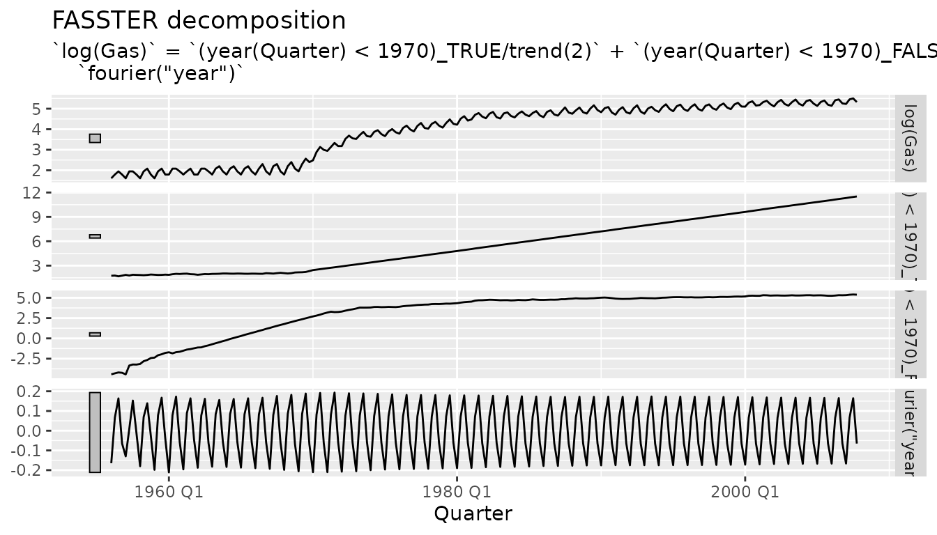

The decomposition reveals: - Original data and fitted values - Level components (separate for pre/post 1970) - Seasonal components

Notice how the pre-1970 level remains flat after 1970, while the post-1970 level takes over, highlighting the structural break.

Forecasting

Generate forecasts using the fitted model:

# Forecast test period
fc <- forecast(fit, h = "5 years")

# Plot forecasts
autoplot(fc, train)

The forecasts: - Use the post-1970 pattern for future predictions - Include uncertainty intervals that grow over time - Capture both trend and seasonal patterns learned from the data

Handling missing values

FASSTER handles missing values naturally during estimation. The Kalman filter simply skips updating states when data is missing:

# Model works even with missing values
data_with_na <- gas_data |>
  # Insert some missing values randomly
  mutate(Gas = if_else(row_number() %in% sample(n(), 10), NA_real_, Gas))

fit_na <- data_with_na |>
  model(FASSTER(Gas ~ (year(Quarter) < 1970) %S% trend(2) + fourier("year", K = 2)))

# Interpolate missing values
fit_na |> 
  interpolate(data_with_na)
#> # A tsibble: 218 x 2 [1Q]
#>    Quarter   Gas
#>      <qtr> <dbl>
#>  1 1956 Q1   5  
#>  2 1956 Q2   6  
#>  3 1956 Q3  23.6
#>  4 1956 Q4   6  
#>  5 1957 Q1   5  
#>  6 1957 Q2   7  
#>  7 1957 Q3  22.1
#>  8 1957 Q4   6  
#>  9 1958 Q1   5  
#> 10 1958 Q2   7  
#> # ℹ 208 more rows

Advanced features

Multiple switching levels

Create complex models with nested switching:

# Different patterns for working days and rainy days
FASSTER(y ~ workday %S% (trend(1) + rain %S% fourier("day")))

Combining components

Mix grouped and ungrouped components:

# Shared trend, separate seasonality
FASSTER(y ~ poly(2) + workday %S% fourier("day"))

Adding ARMA terms

Correct for remaining autocorrelation:

# Add AR(1) term
FASSTER(y ~ workday %S% (poly(1) + fourier("day")) + ARMA(ar = c(0.8, -0.3), ma = 0.4))

Parameter estimation

FASSTER uses a heuristic approach for fast parameter estimation:

Filter data with default parameters
Smooth states to approximate desired behavior
Extract variances from smoothed states
Use estimated parameters for final model

This “filterSmooth” approach: - Requires only two passes through the data - Works well with non-saturating Fourier terms - Provides reasonable estimates without maximum likelihood

For very long series, estimation can be sped up by using only recent data:

# Use only last 1000 observations for parameter estimation
FASSTER(y ~ model, include = 1000)

Summary

FASSTER provides a flexible framework for modeling complex time series with:

Modular component specification
State switching for irregular multiple seasonality
Fast estimation via Kalman filtering
Natural handling of missing values
Model-based decomposition

The concise formula interface makes it easy to specify models suitable for high-frequency data with complex seasonal patterns.